Master's Degree Thesis:
Overcoming the limits of Deep Reinforcement Learning with Model-Based approach
Realized in 2020 Tags: Model-based, deep reinforcement learning, deep learning, planet, neural network
Presentation:
 Hi everyone, I'm Luca Sorrentino, and this is my master's thesis work discussion.
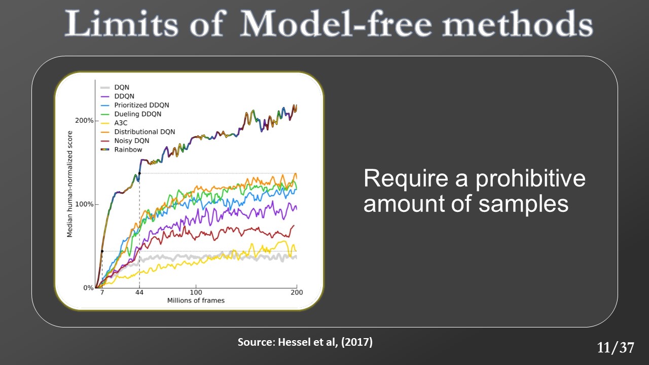
This work focused on identifying the model-based technique for overcoming the limits of model-free Deep Reinforcement Learning.
This work was done at Addfor s.p.a., which is a company that produces Artificial Intelligence solutions.
Hi everyone, I'm Luca Sorrentino, and this is my master's thesis work discussion.
This work focused on identifying the model-based technique for overcoming the limits of model-free Deep Reinforcement Learning.
This work was done at Addfor s.p.a., which is a company that produces Artificial Intelligence solutions.
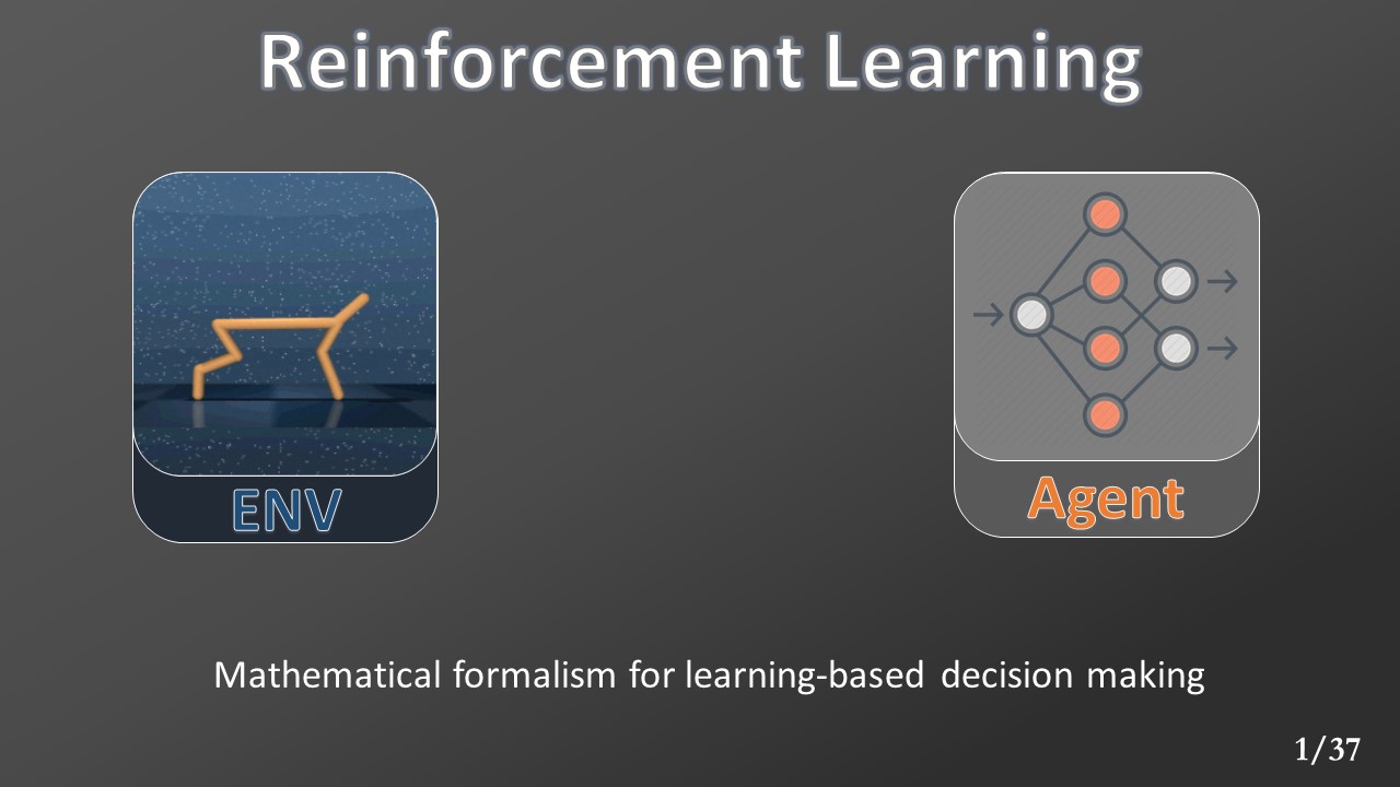 Reinforcement learning is a mathematical formalism for learning-based decision-making.
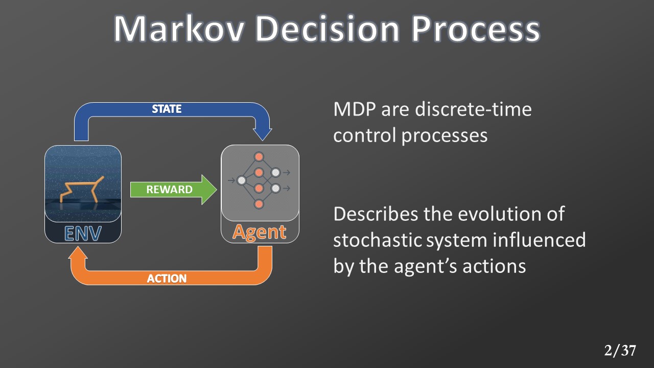 This method is used to train an agent to achieve a goal without supervision. The agent will compute actions, and for each of them, it receives a feedback signal called “reward.” The environment is formalized with a Markov Decision Process (MDP).
An MDP describes the evolution, at a discretized time, of a stochastic system influenced by an agent.
This method is used to train an agent to achieve a goal without supervision. The agent will compute actions, and for each of them, it receives a feedback signal called “reward.” The environment is formalized with a Markov Decision Process (MDP).
An MDP describes the evolution, at a discretized time, of a stochastic system influenced by an agent.
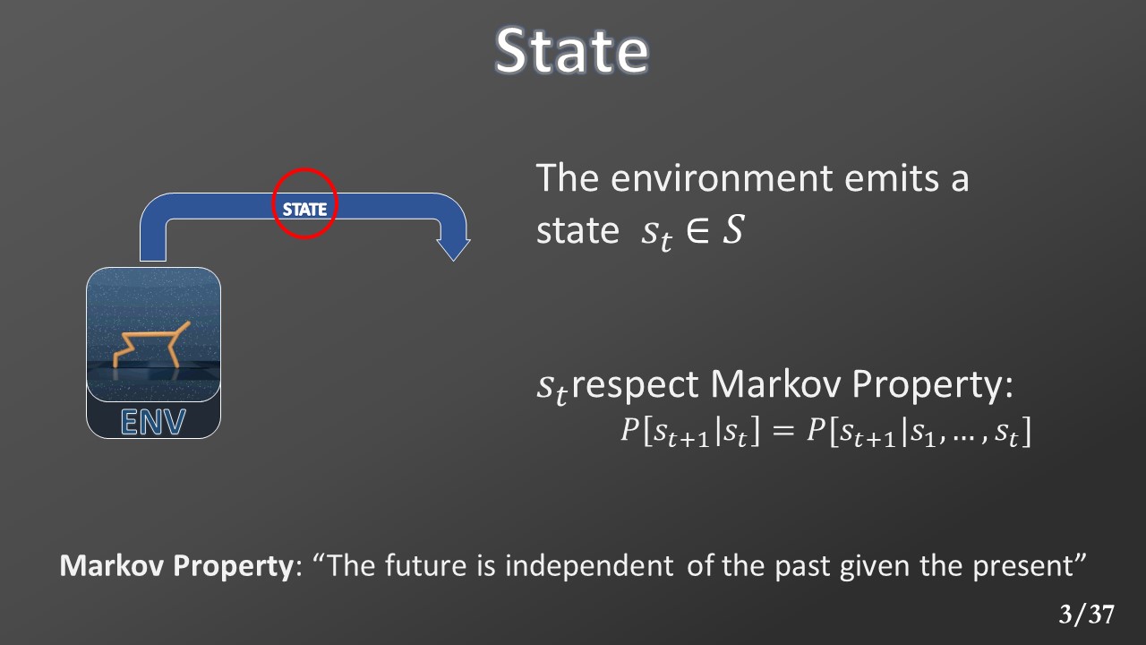 At each time step t, the environment collects all the current state’s main information in a vector “s”. This vector must respect the Markov Property, so maintain enough data to allow the successive state’s prediction without looking into history.
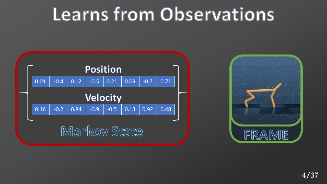 To respect the Markov property, a domain expert must analyze the task and manually individuate all the essential information to collect during the environment construction. We can avoid this by providing only partial information to the agent, an observation derived from the real state. For example, a frame from the camera or images rendered by the simulator. This makes the learning process harder since the agent must find, collect, and keep in memory all the information by itself. In this work, we will see how to train an agent efficiently in pixel space directly.
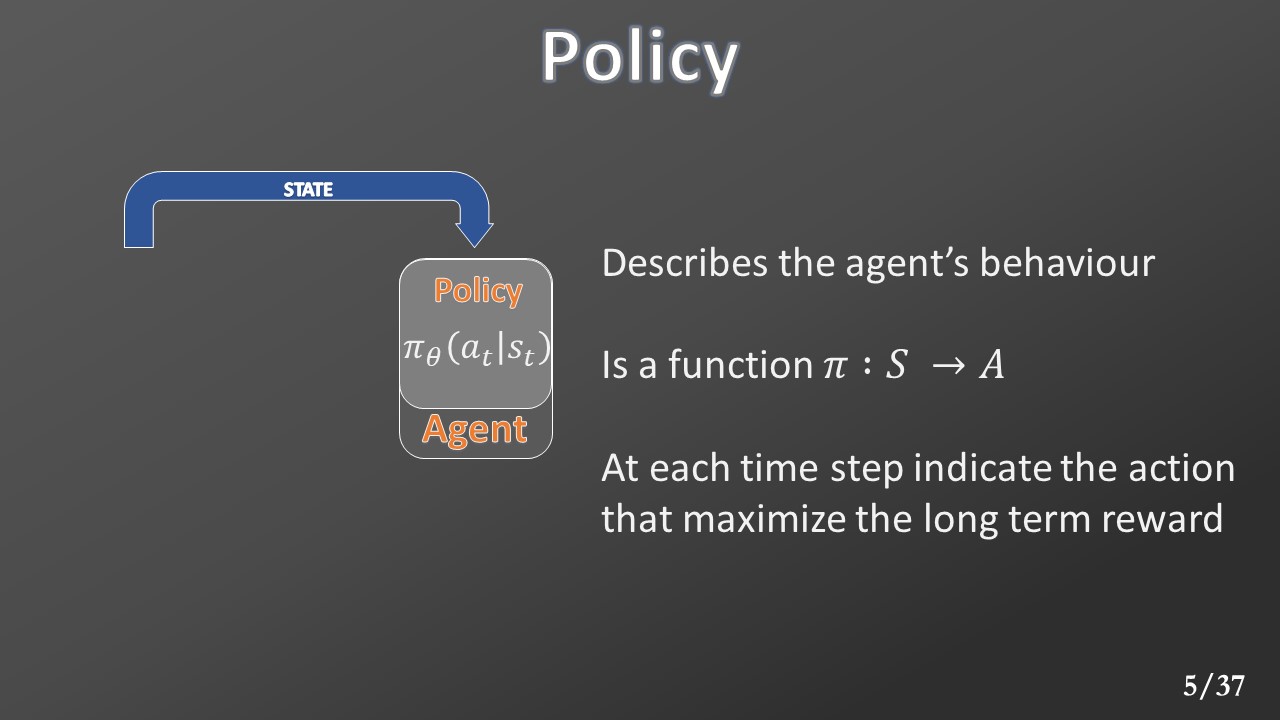 When the agent receives a State, it invokes its policy that describes the agent’s behavior mapping the state space to the action space. For each state in input, it provides the respective action that maximizes the long-term reward.
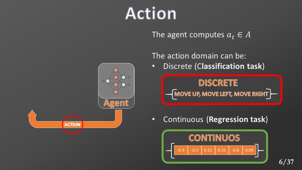 The action space could be discrete (requiring a classification task) or continuous (requiring a regression task). In this work, all the experiments are computed on environments with continuous domain action.
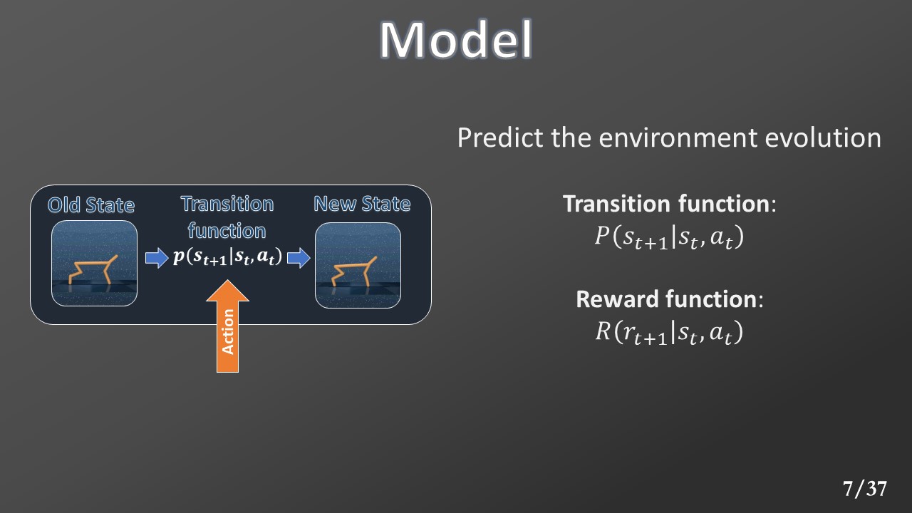 Once the environment receives the action, it calls the model. A model comprises two functions: the transition function that maps the current state and action to a distribution of the possible new state (the environment is stochastic) and a reward function that generates a reward from the current state and action.
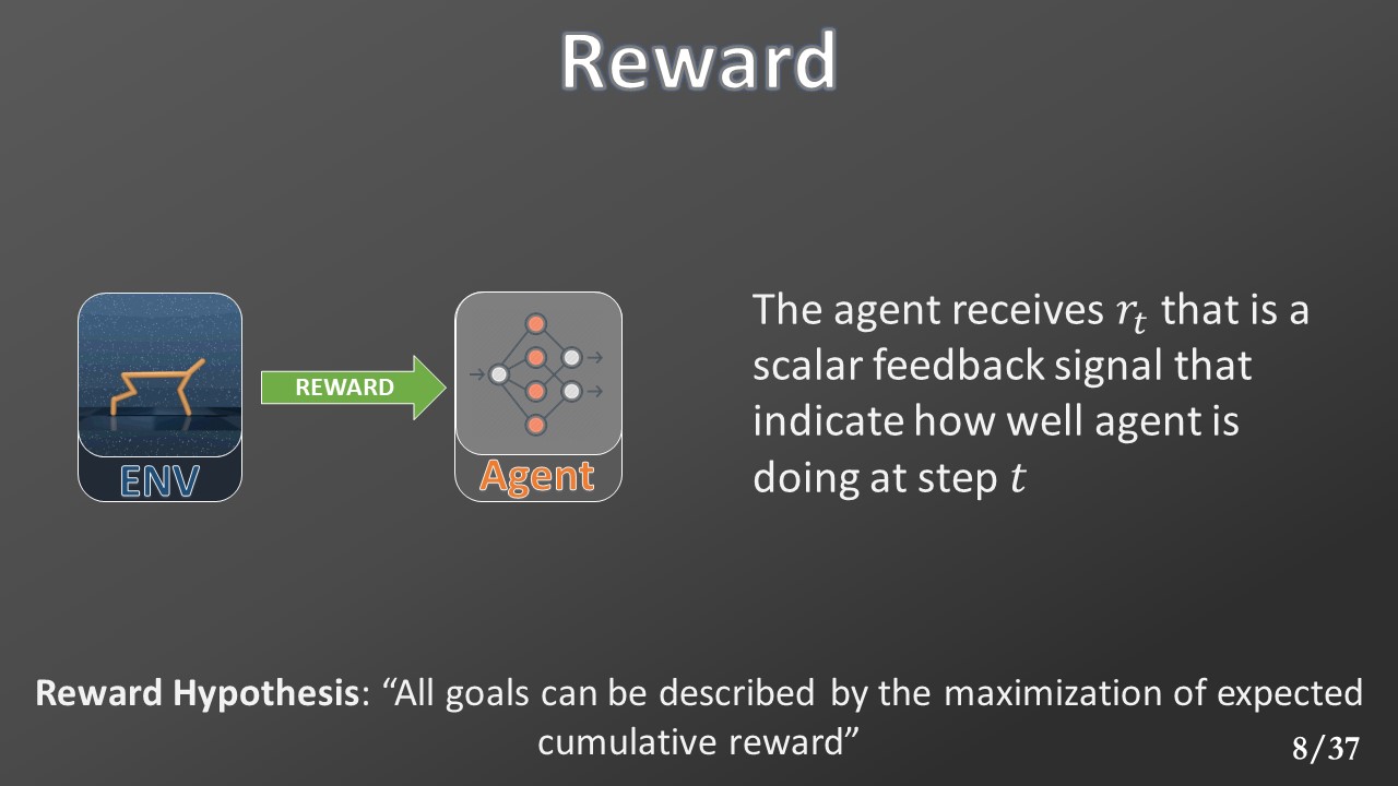 The reinforcement learning framework is based upon the reward hypothesis that “the maximization of expected cumulative reward can describe all goals.”
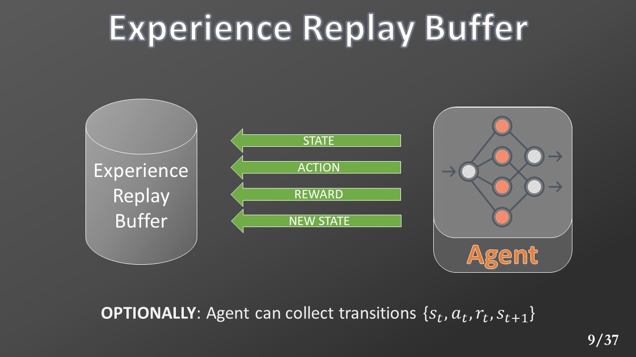 Lastly, an agent can collect all the transitions [state, action, reward, new_state] in an experience replay buffer.
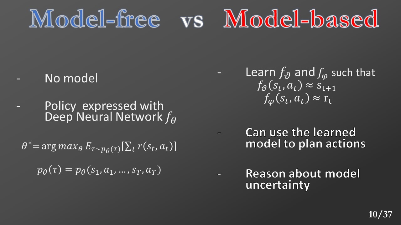 Now we can introduce the concept of model-free e model-based deep reinforcement learning. In the first case, the algorithm does not explicitly build the environment model, but they represent the policy with a deep neural network trained to map an action to the state directly. With the model-based approach, the agent uses the deep neural network to approximate both the transition and reward functions. Then it can use this information to represent the policy with a planner.
 Now we can introduce the concept of model-free e model-based deep reinforcement learning. In the first case, the algorithm does not explicitly build the environment model, but they represent the policy with a deep neural network trained to map an action to the state directly. With the model-based approach, the agent uses the deep neural network to approximate both the transition and reward functions. Then it can use this information to represent the policy with a planner.
 Let’s start to talk about the model-based algorithm chosen for this master thesis. It is called PLAnning NETwork (PlaNet), it was published by Danija et al. in 2019, and it is still considered a state-of-the-art method for model-based DRL.
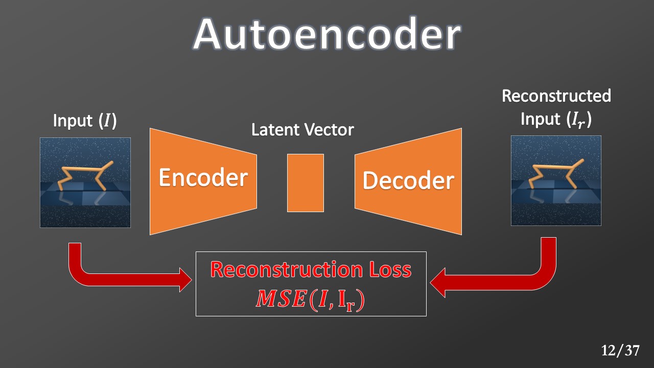 It is heavily based on Autoencoder’s idea, where input is compressed into a latent vector and then reconstructed. The model is trained to minimize a loss function called “reconstruction loss”. This loss is calculated as a distance between the original input and the reconstruction. This process guarantees that the model will capture all the salient features into the latent vector.
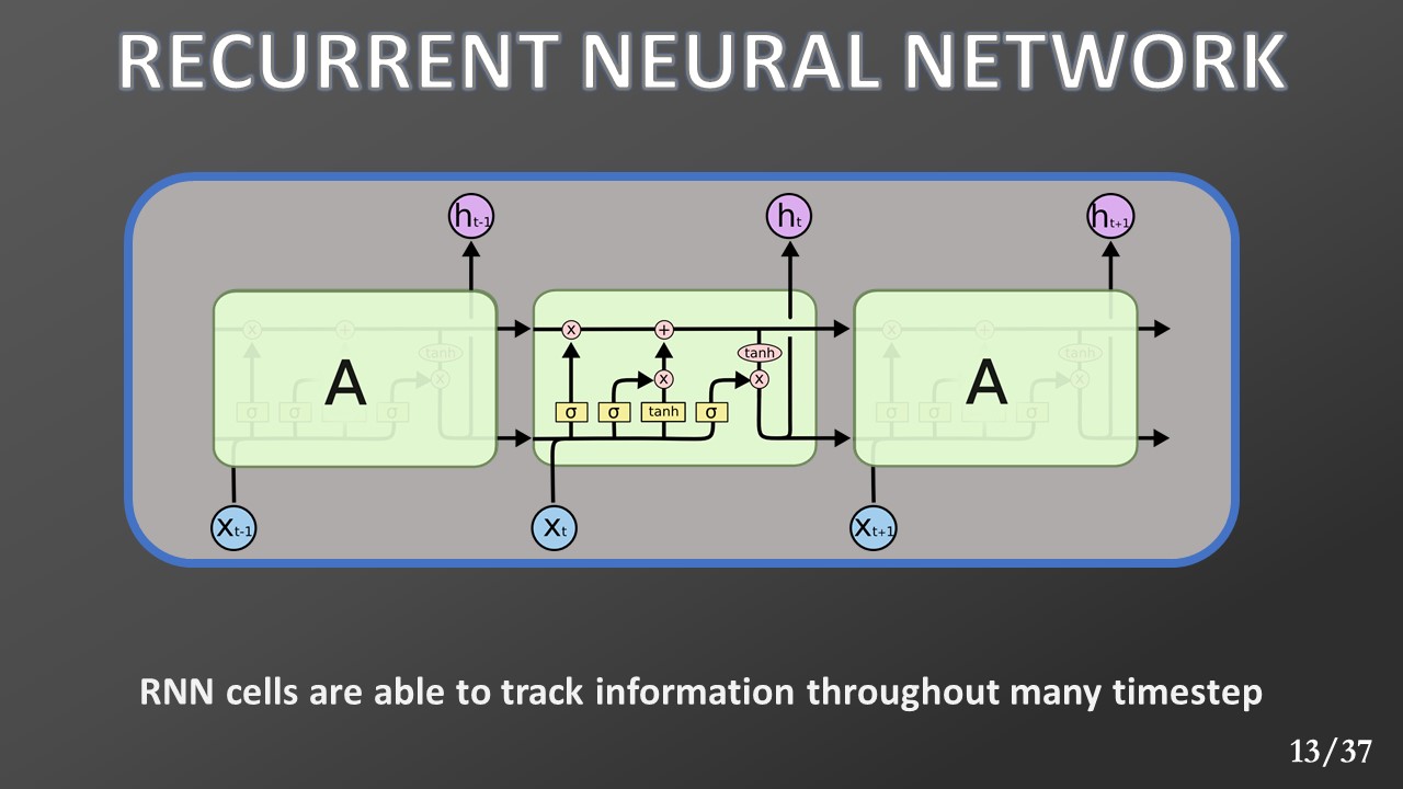 Since we decided not to respect Markov property, an RNN is used to reconstruct it. The Recurrent Neural Network (RNN) can track information throughout many time steps, providing the current input a temporal context. In other words, it is able to reconstruct the state's history.
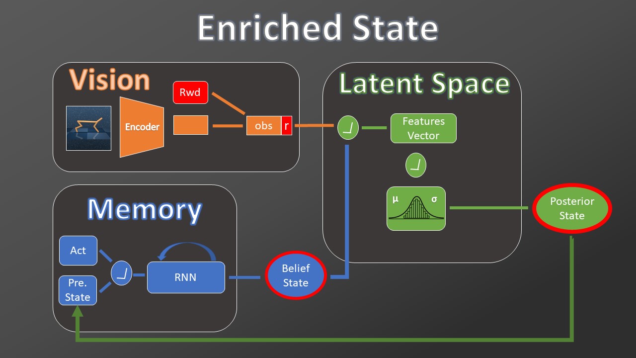
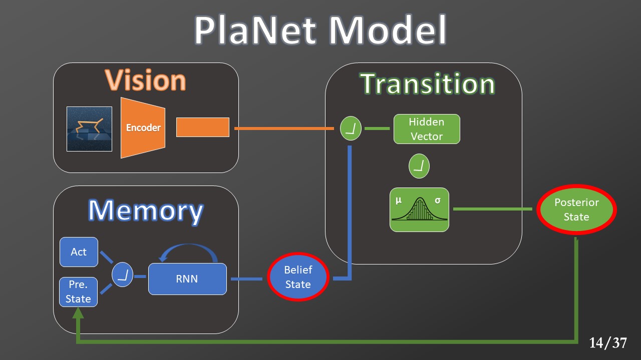 PlaNet model is composed of three submodules:
The vision module uses a convolutional network to encode in a single vector all the input visual information.
The memory module receives information about the current action to take and the precedent states. Then it uses a Gated Recurrent Unit (GRU) to encode the received data in the Belief State vector.
Next, both the two vectors are sent to the Transition modules where a feedforward network will produce the Gaussian distribution parameters. This Gaussian will be an approximation of the one created by the environment transition model. From this Gaussian will be sampled a vector, called Posterior State.
PlaNet model is composed of three submodules:
The vision module uses a convolutional network to encode in a single vector all the input visual information.
The memory module receives information about the current action to take and the precedent states. Then it uses a Gated Recurrent Unit (GRU) to encode the received data in the Belief State vector.
Next, both the two vectors are sent to the Transition modules where a feedforward network will produce the Gaussian distribution parameters. This Gaussian will be an approximation of the one created by the environment transition model. From this Gaussian will be sampled a vector, called Posterior State.
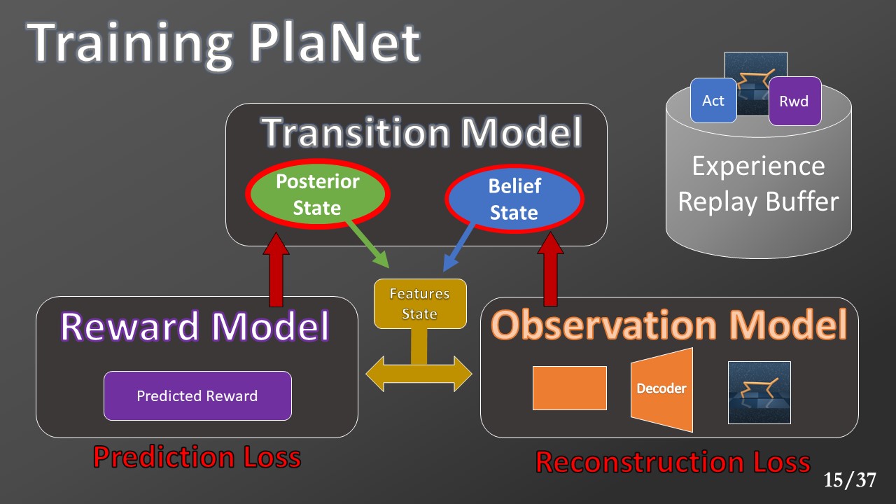 The Posterior and the Belief State’s concatenation leads to the Markovian State’s approximation that we called Features State. The reward model uses this state and the current action to predict the reward. The Observation Model uses this state to recreates the current observation (the same provided in input).
Both these models are trained to minimize the Mean Squared Error (MSE) with respect to the data collected in the experience replay buffer.
The Posterior and the Belief State’s concatenation leads to the Markovian State’s approximation that we called Features State. The reward model uses this state and the current action to predict the reward. The Observation Model uses this state to recreates the current observation (the same provided in input).
Both these models are trained to minimize the Mean Squared Error (MSE) with respect to the data collected in the experience replay buffer.
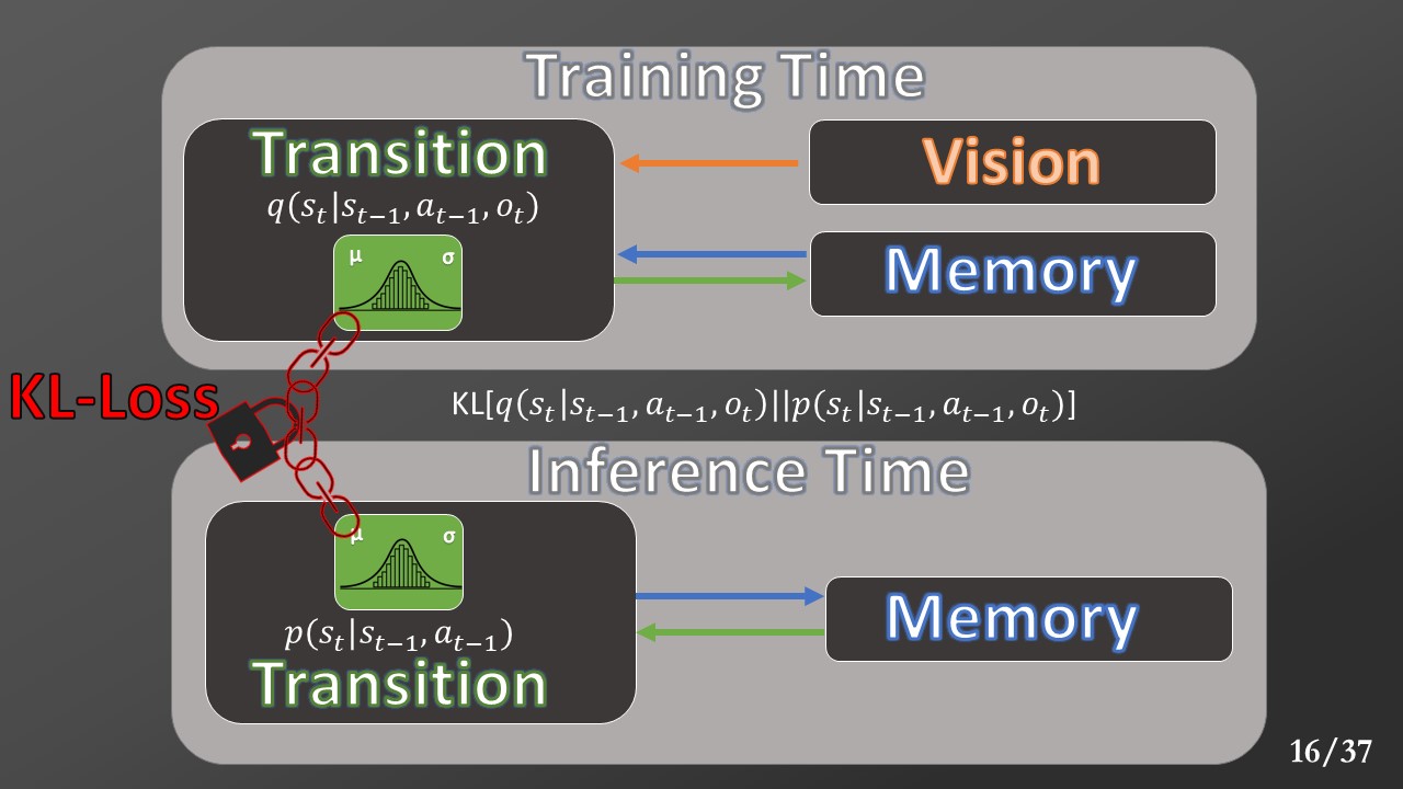 Even if this model works well at training time, we can’t use it at inference time. If we want to ask the model to make predictions, we only can provide him the previous state and the action that we would take. We would use another model at inference time that does not require the current observation (we remove the vision module). Even if we provide less information to this new model, we would say that the transition model maintains the same result like the one used ad training time. To reach this goal, we apply a KL-loss to bring the two distributions closer together. The KL-loss calculates the amount of information that can be lost using one distribution to approximate another one.
 Now we have a model that is able to predict the future. Let’s see how we can use it to plan the action to take.
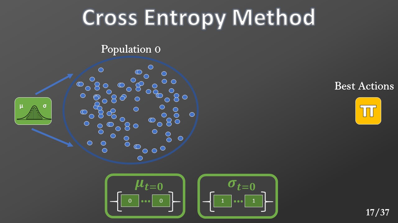 The planner is based on a genetic algorithm called Cross-Entropy Method (CEM). We define the “plan” as a list of actions. At each a “plan population.” The Gaussian parameters are initialized with zero mean and one variance.
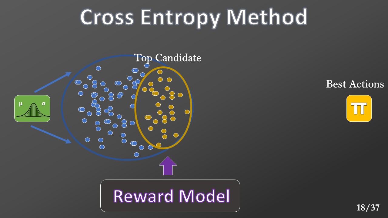 The approximated reward model is then used to find the population’s elites (top candidate) that maximize the expected reward.
 The top candidate will be used to calculate the new Gaussian parameters for the next generation.
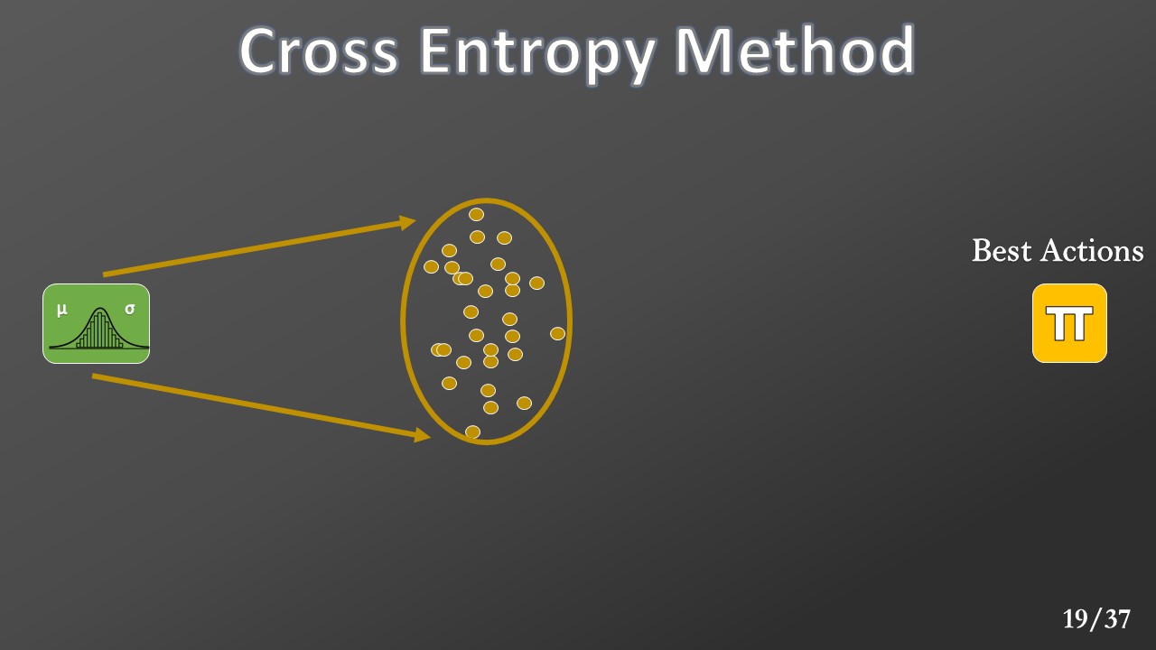
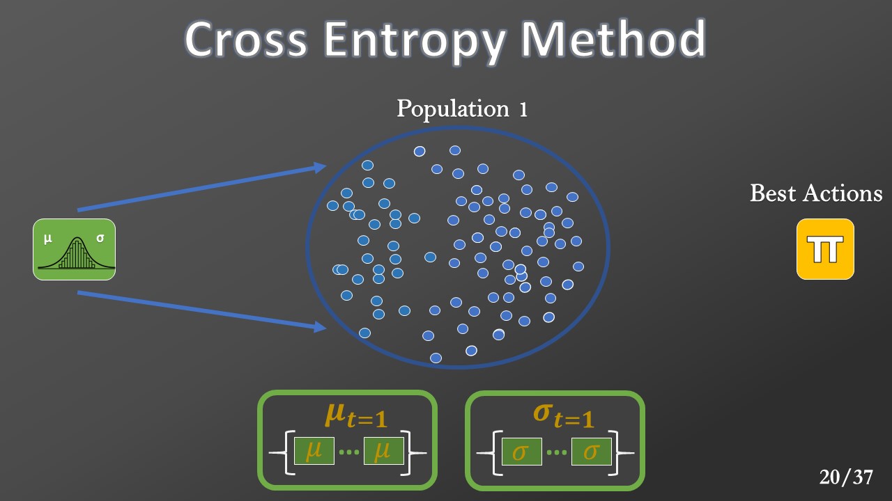 This optimization procedure is repeated for a few iterations. The final action is the mean of the top candidate of the last generated population.
 Now that we have finished explaining the model let’s see our experiments.
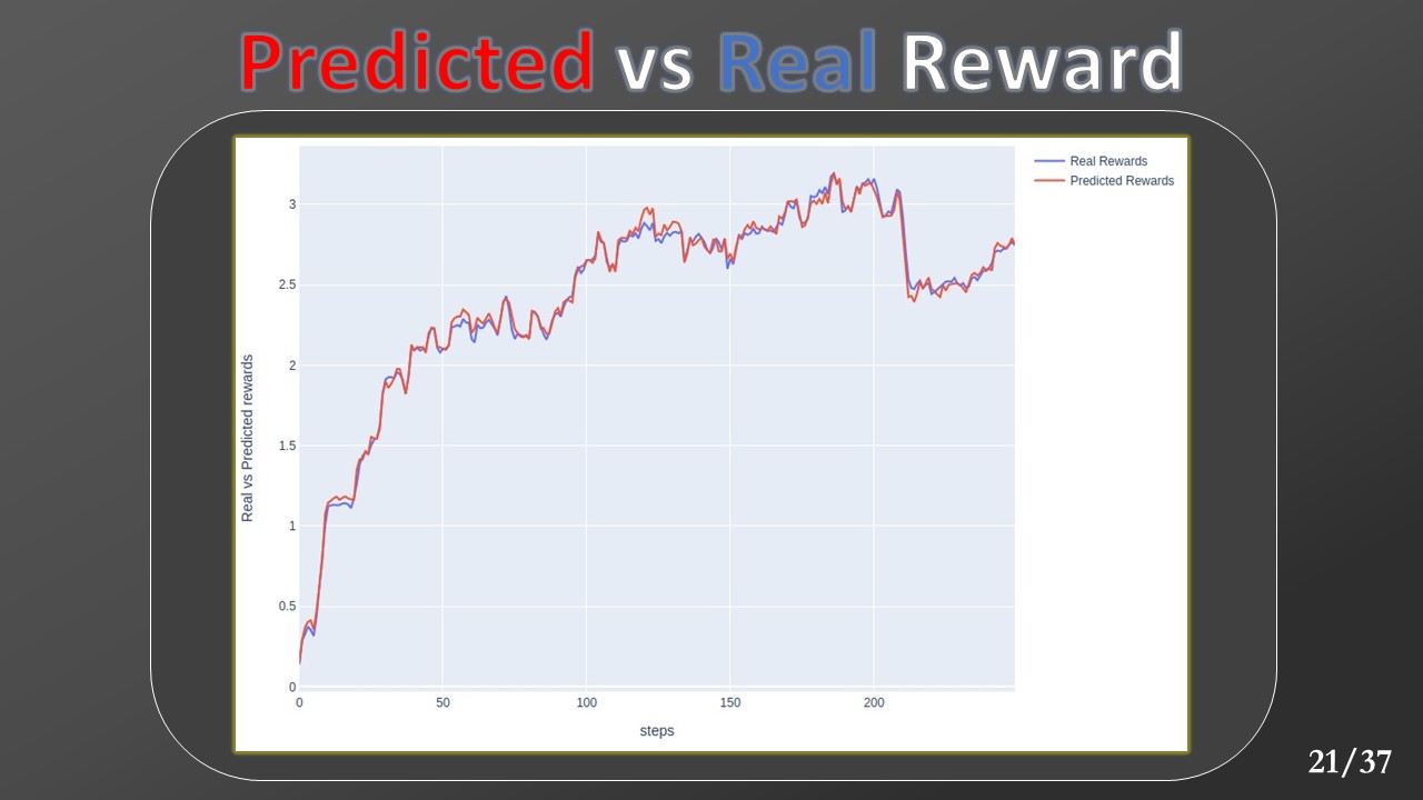 Let's start with the reward prediction. In this plot, the red line represents the predicted reward value, and the blue line the received reward. We can see how the model is able to correctly approximate the real reward function for all the steps of the episode.
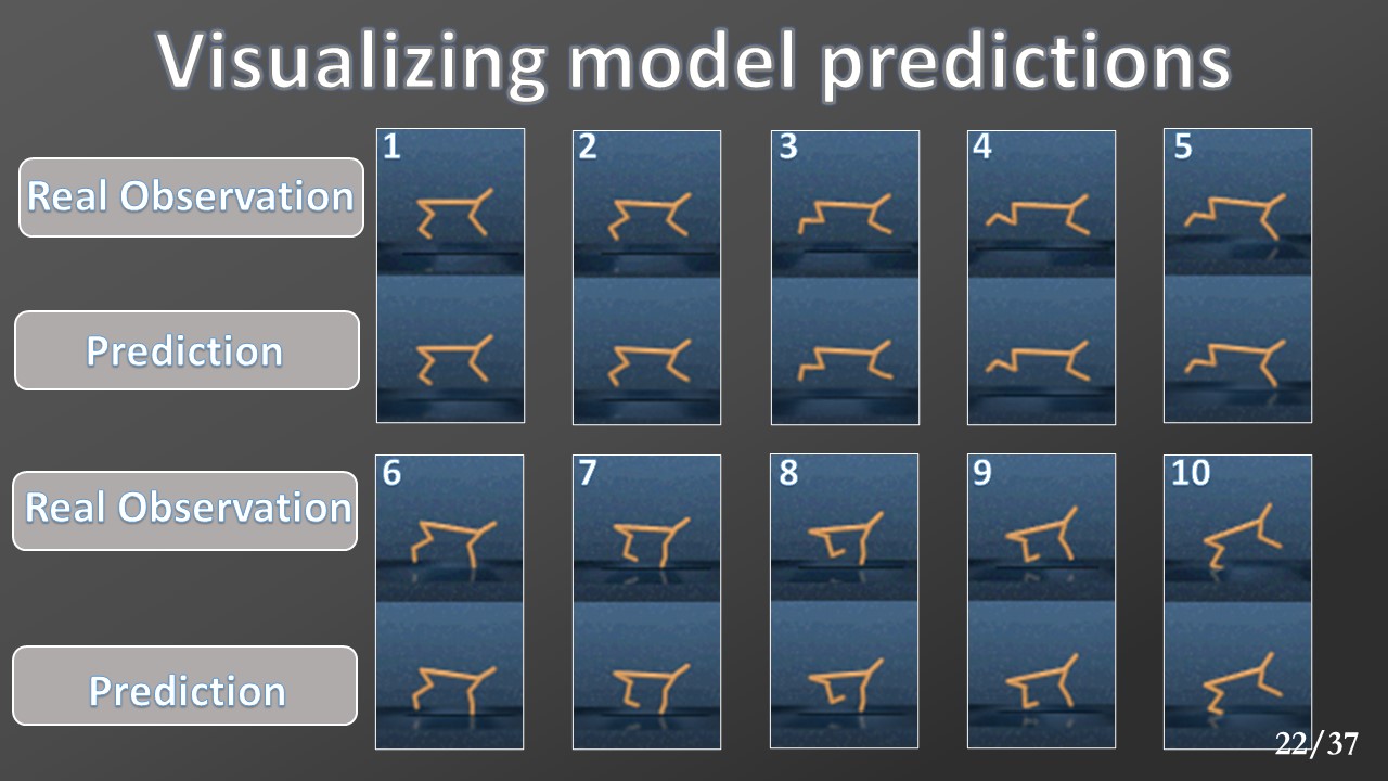 Let's now analyze the model ability of frame prediction and reconstruction. In this experiment, the agent receives a single observation as input, and it must predict the remaining ten.
For each prediction, you can see the corresponding real observation placed above it. Let's see how, even in this case, the predictions are compelling for all ten steps above.
Let's now analyze the model ability of frame prediction and reconstruction. In this experiment, the agent receives a single observation as input, and it must predict the remaining ten.
For each prediction, you can see the corresponding real observation placed above it. Let's see how, even in this case, the predictions are compelling for all ten steps above.
 We extended the planning horizon to show how the errors pile up when the predictions go on. Two errors are particularly evident in the frame 12 and 14 where the cheetah's hind legs are not perfectly aligned.
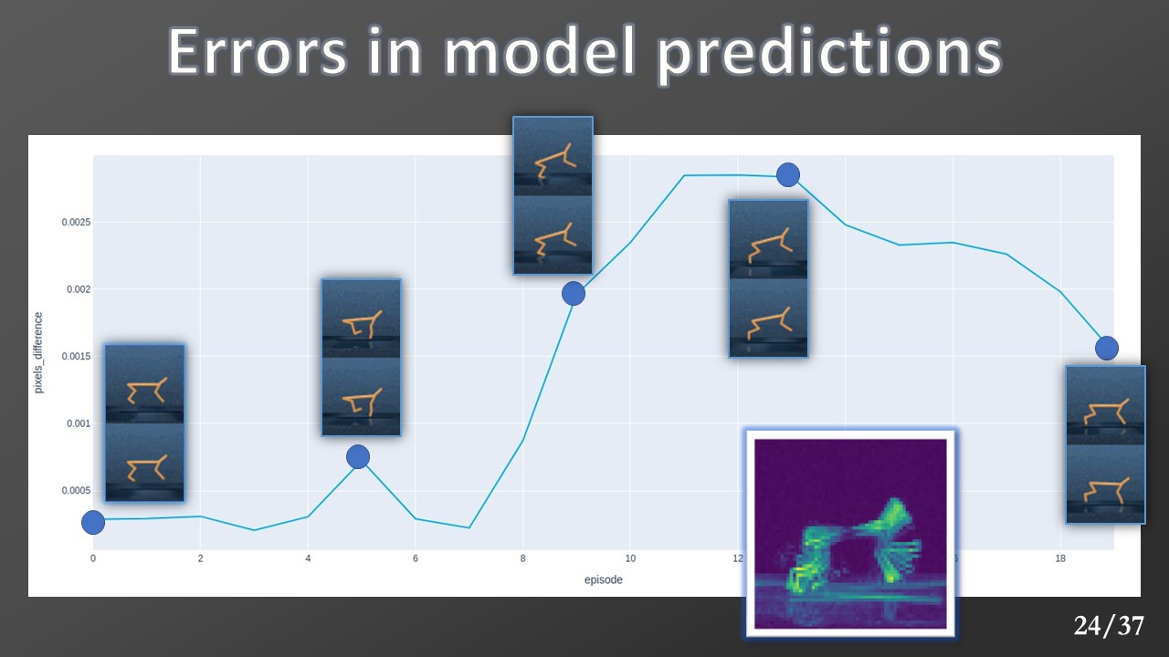 We realized this plot where the y-axis value is calculated with an MSE between the real observations and the predicted ones to have a more quantitative comparison. This plot confirms the previous result, and it can be used to find the best prediction horizon. We also produced a heatmap to highlight the area where the model computes the most errors. As we could expect, the heatmap shows that the model makes more errors in the hind and front legs of the cheetah and the head’s zone.
 Let’s talk now about some experimental improvements applied to the original model.
 The first one is an implementation detail. The original implementation uses a command to reduce the observation resolution to [64,64] pixels. During this process, they lost a lot of information. We discovered how to render directly to the desired resolution, achieving a great boost in our results.
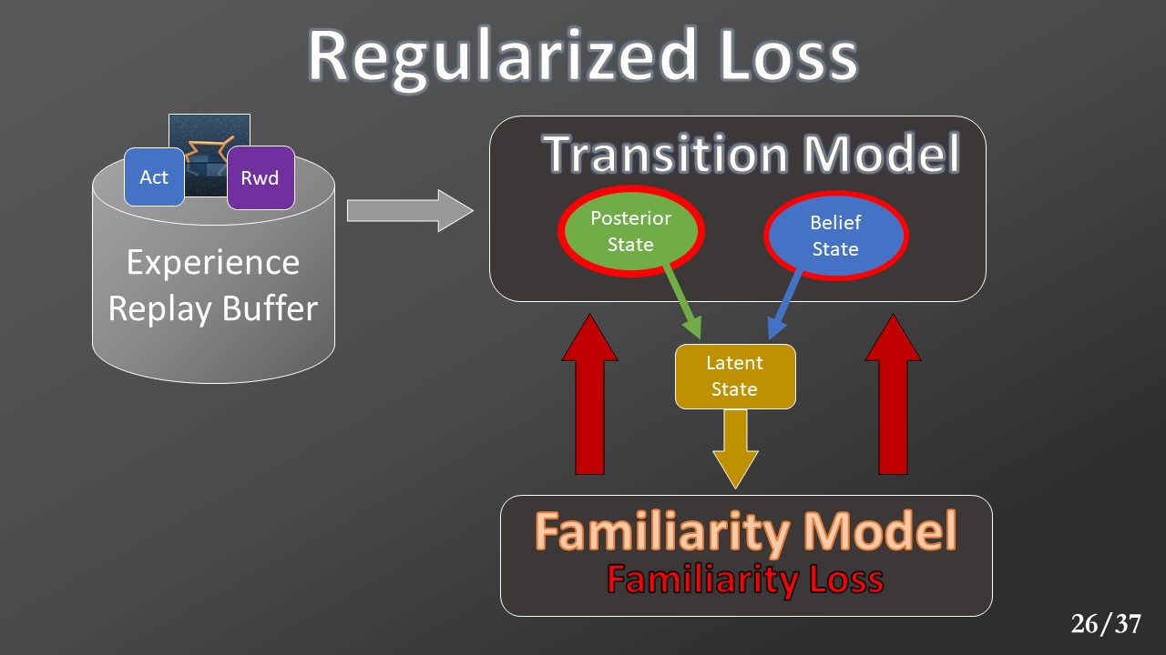 Next, we modified the model architecture adding a new loss from a regularizer model. With this new loss, which we call “familiarity loss,” the transition model's predictions are further penalized when they move away from the distribution of the data collected in the experience buffer, pushing the model to stick as much as possible to what it actually saw during its explorations.
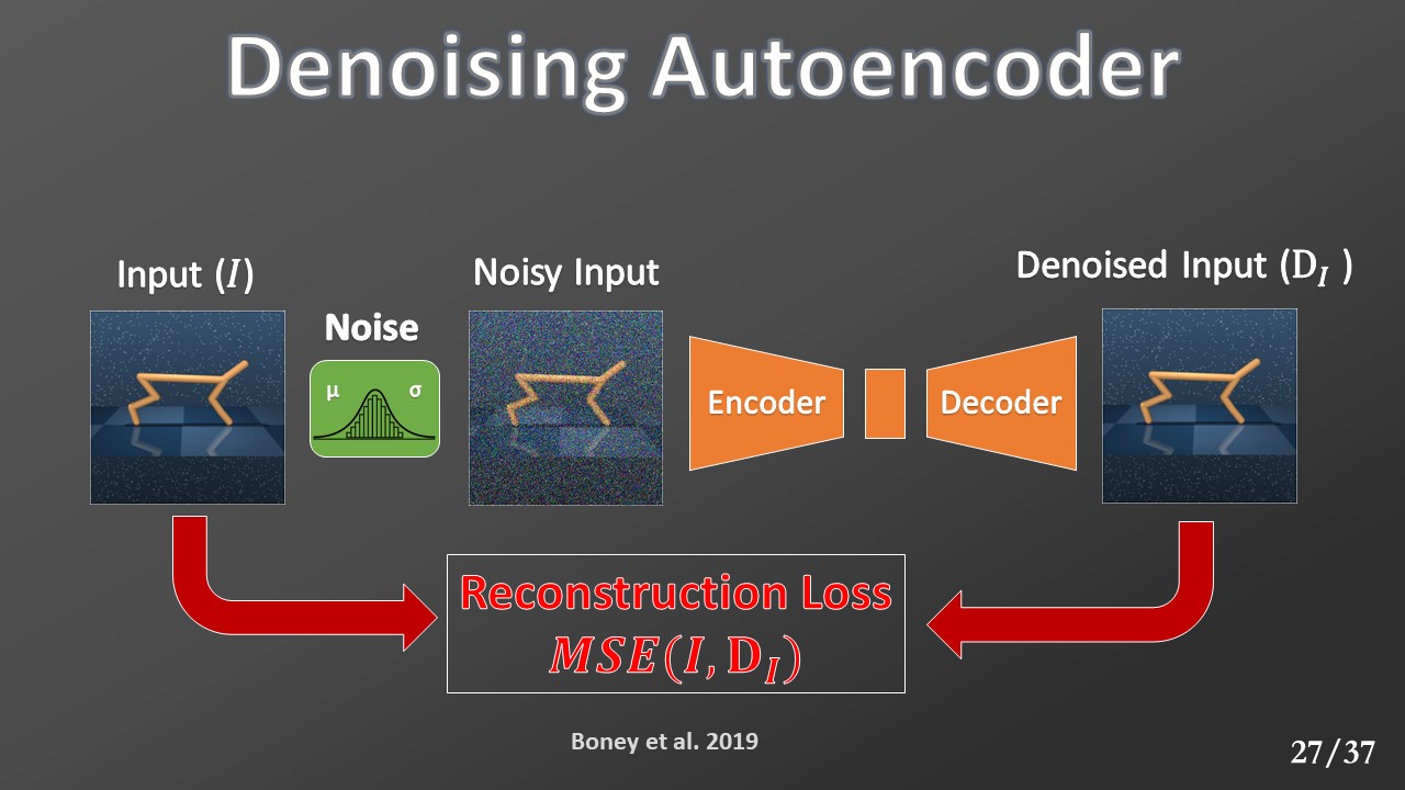 To do this, we have trained A denoising autoencoder that is a modified version of the autoencoder in which Gaussian noise is added to the input before it is sent to the model. However, this model’s loss is calculated with respect to the model's ability to reconstruct the original input to remove the added noise.
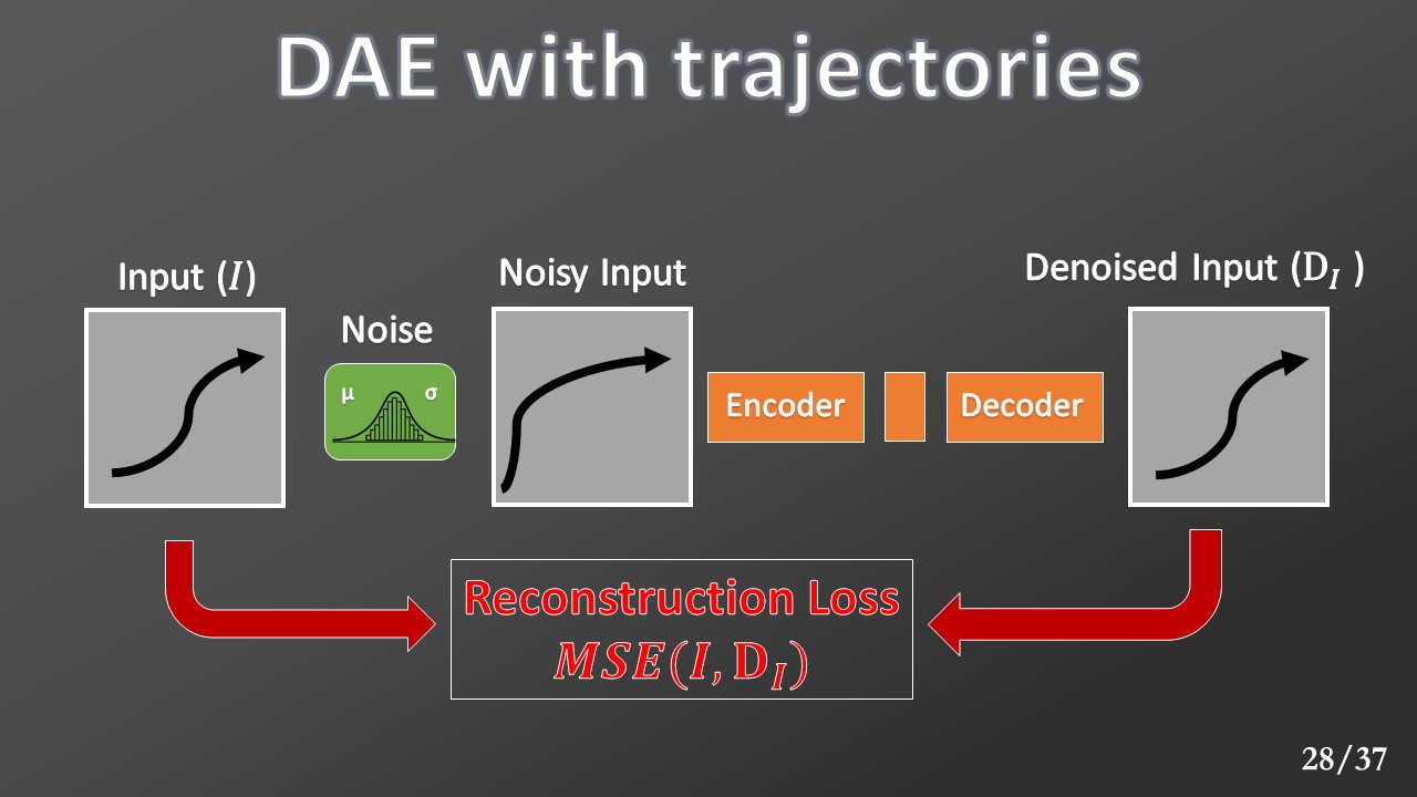 In this case, the model provided input is the sequence of "state, action, a new state, new action etc. " These sequences are called “trajectories,” and their length corresponds to the prediction horizon.
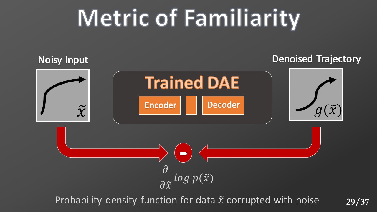 The DAE does not directly learn the distribution of trajectories. It is used to identify the amount of trajectory’s corruption. The more this value is high (means that the provided trajectory is unfamiliar w.r.t the collected ones), the more the loss increments.
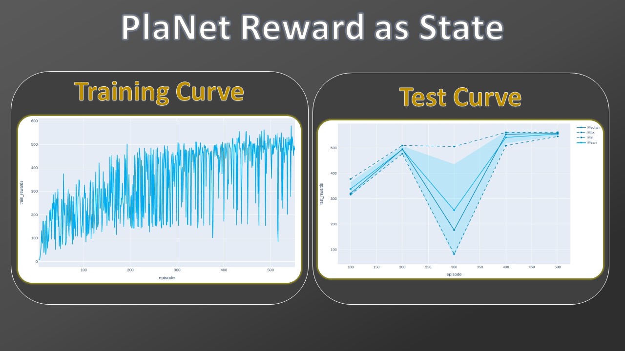
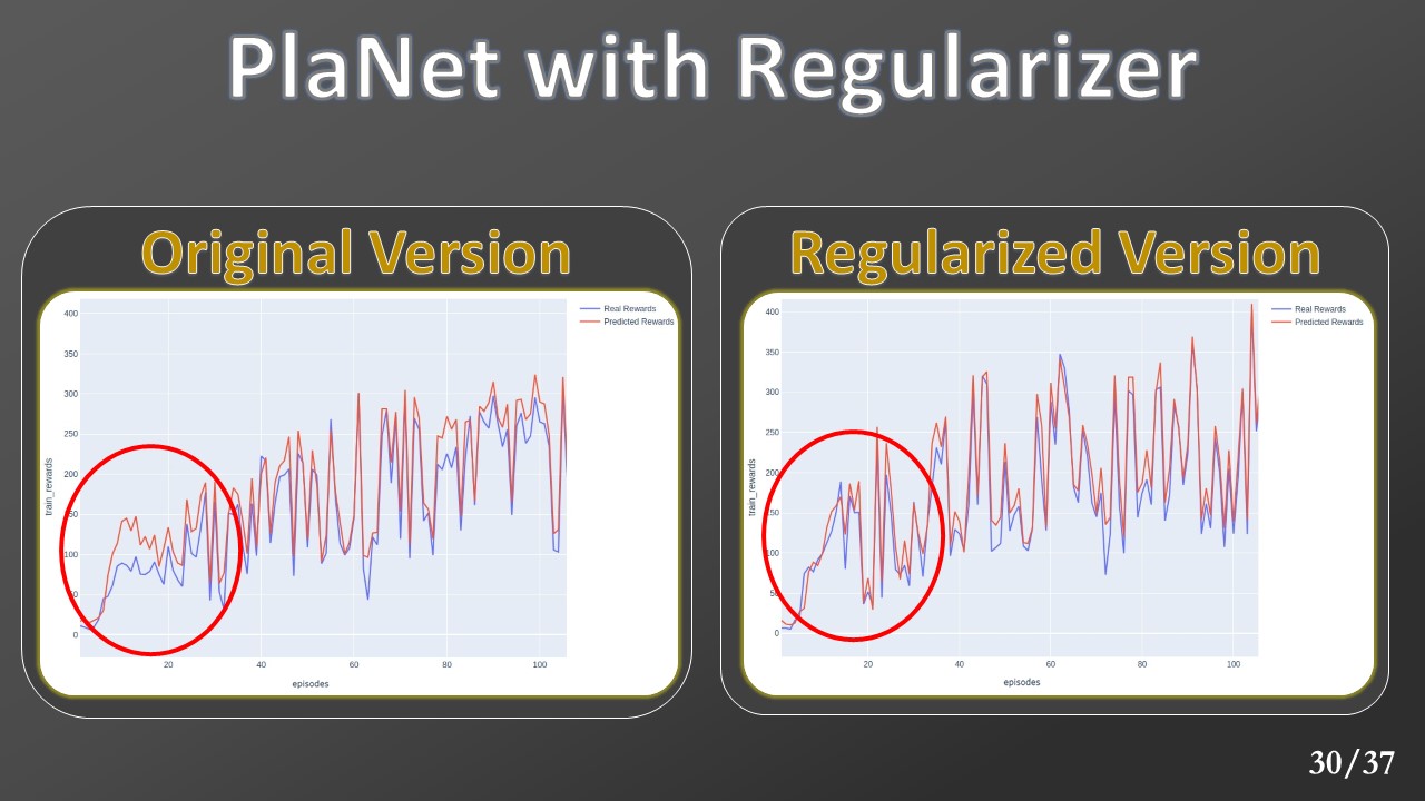 Plotting the cumulative reward for each training episode, we can see the regularized effect (right plot) with respect to the one realized without it (left plot). We note how the predictive gap is removed just from the first episodes.
 Analyzing the obtained rewards, we confirm that the regularizer allows obtaining high rewards from the very first episodes, and then when the accumulated experience grows, its contribution disappears.
The regularizer has provided a promising result and is in line with what appears in the literature, but it needs further experiments to be validated. For time and resource problems, it is tested only in one environment.
Analyzing the obtained rewards, we confirm that the regularizer allows obtaining high rewards from the very first episodes, and then when the accumulated experience grows, its contribution disappears.
The regularizer has provided a promising result and is in line with what appears in the literature, but it needs further experiments to be validated. For time and resource problems, it is tested only in one environment.
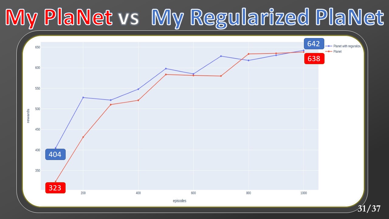
 Let’s now see some comparisons with other model-based and model-free SOA algorithms. ALL THE FOLLOWING PRESENTED RESULTS ARE OBTAINED WITHOUT THE REULARIZER.
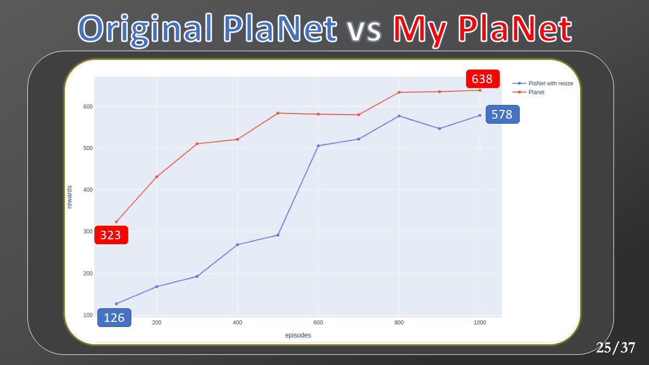
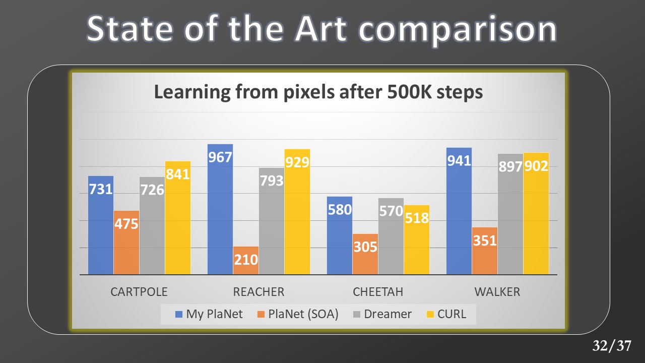 First, we validated our version of Planet’s results with respect to the original one and other state-of-the-art model’s results.
These are the results produced after half a million steps from my planet (in blue), the original planet (in orange), from the evolution of Planet, or dreamer (in gray), and finally from a new system called Contrastive unsupervised representations for reinforcement learning In yellow. The last one is not a model-based system, but I have reported since the data collected comes from that paper in which it is presented. We can see how my planet’s results after 500 steps exceed those of the original version and are comparable to the remaining methods.
First, we validated our version of Planet’s results with respect to the original one and other state-of-the-art model’s results.
These are the results produced after half a million steps from my planet (in blue), the original planet (in orange), from the evolution of Planet, or dreamer (in gray), and finally from a new system called Contrastive unsupervised representations for reinforcement learning In yellow. The last one is not a model-based system, but I have reported since the data collected comes from that paper in which it is presented. We can see how my planet’s results after 500 steps exceed those of the original version and are comparable to the remaining methods.
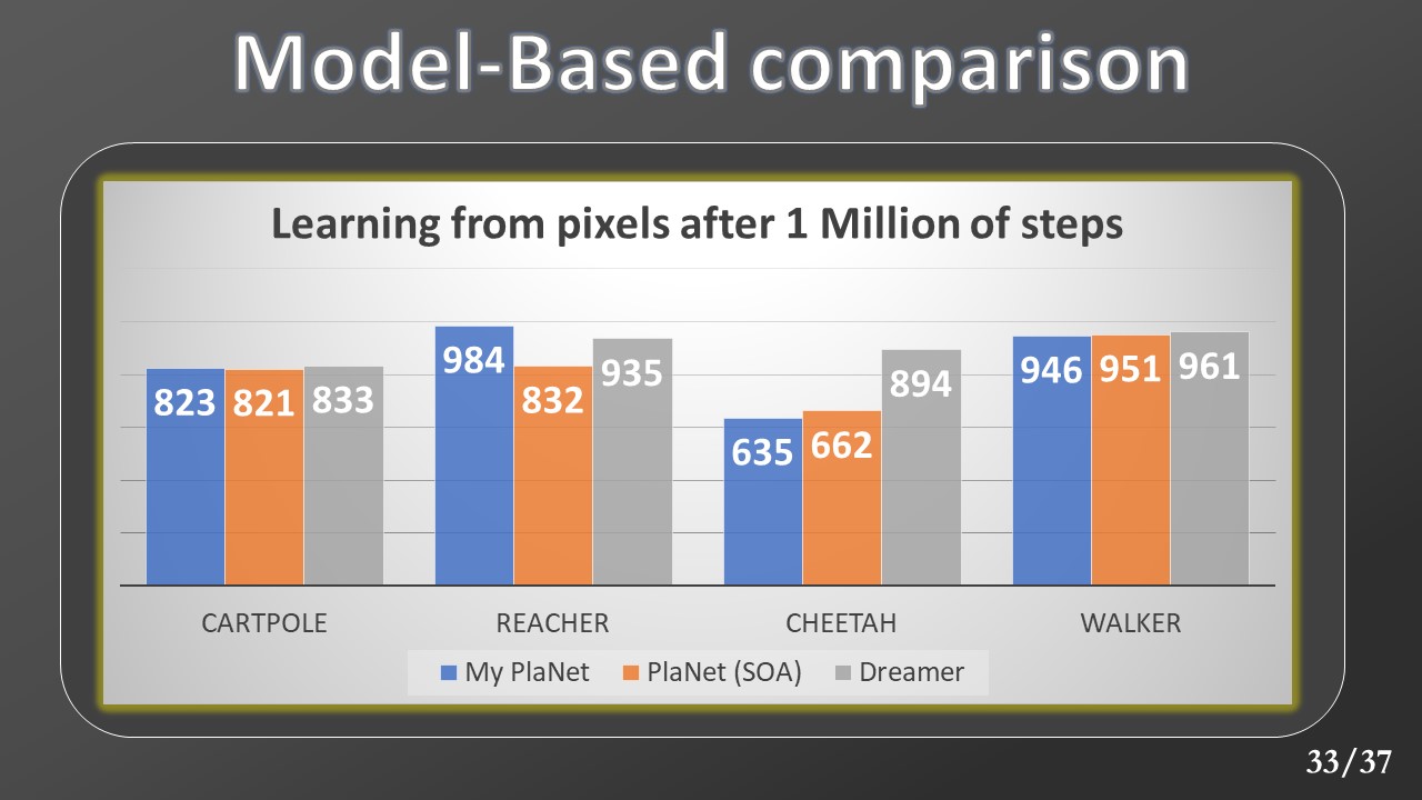 By bringing the number of steps to one million, the results remain in line with those of the original model.
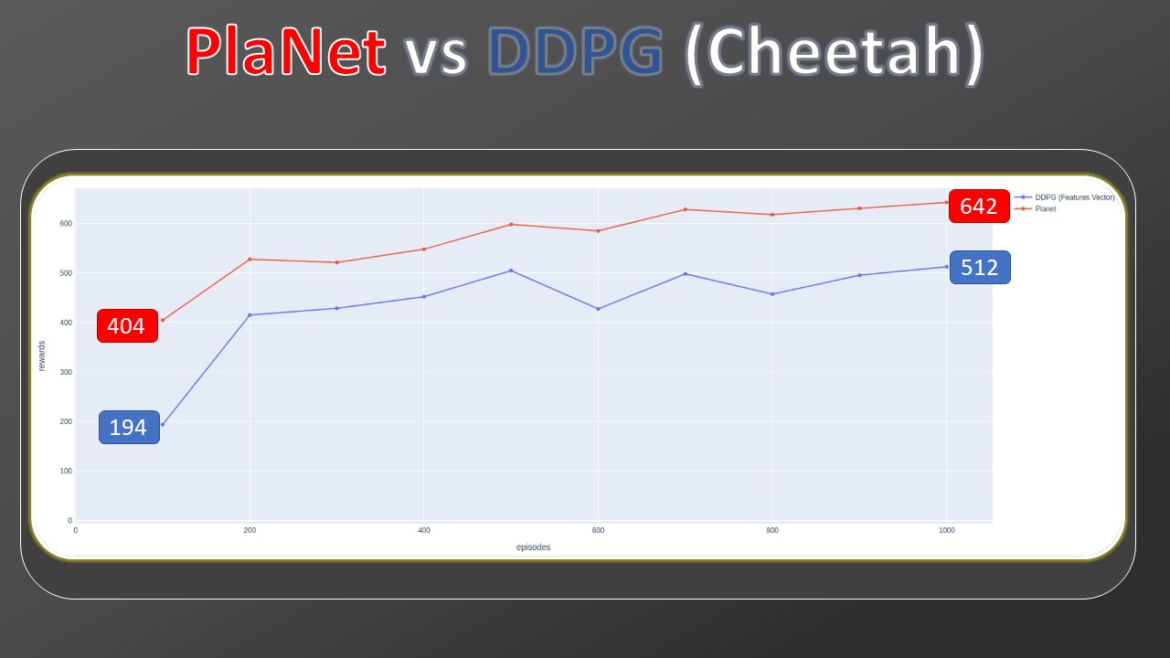
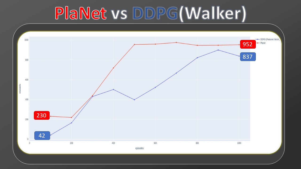
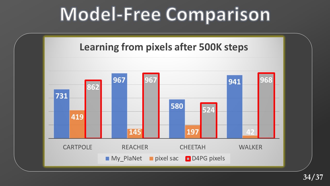 At this point, we move on to the comparison with model-free algorithms. In this graph, we can see the results of my Planet (in blue) compared to those of a model-free algorithm called SAC (in orange). The results were produced after a 500k step training which took place directly in pixels space. Let's see how Planet surpasses SAC in all 4 environments. In the gray bar instead, we observe the results of another model-free algorithm called D4PG trained for 100M of steps. Despite a number of samples of orders of magnitude higher, we observe how the results are still comparable.
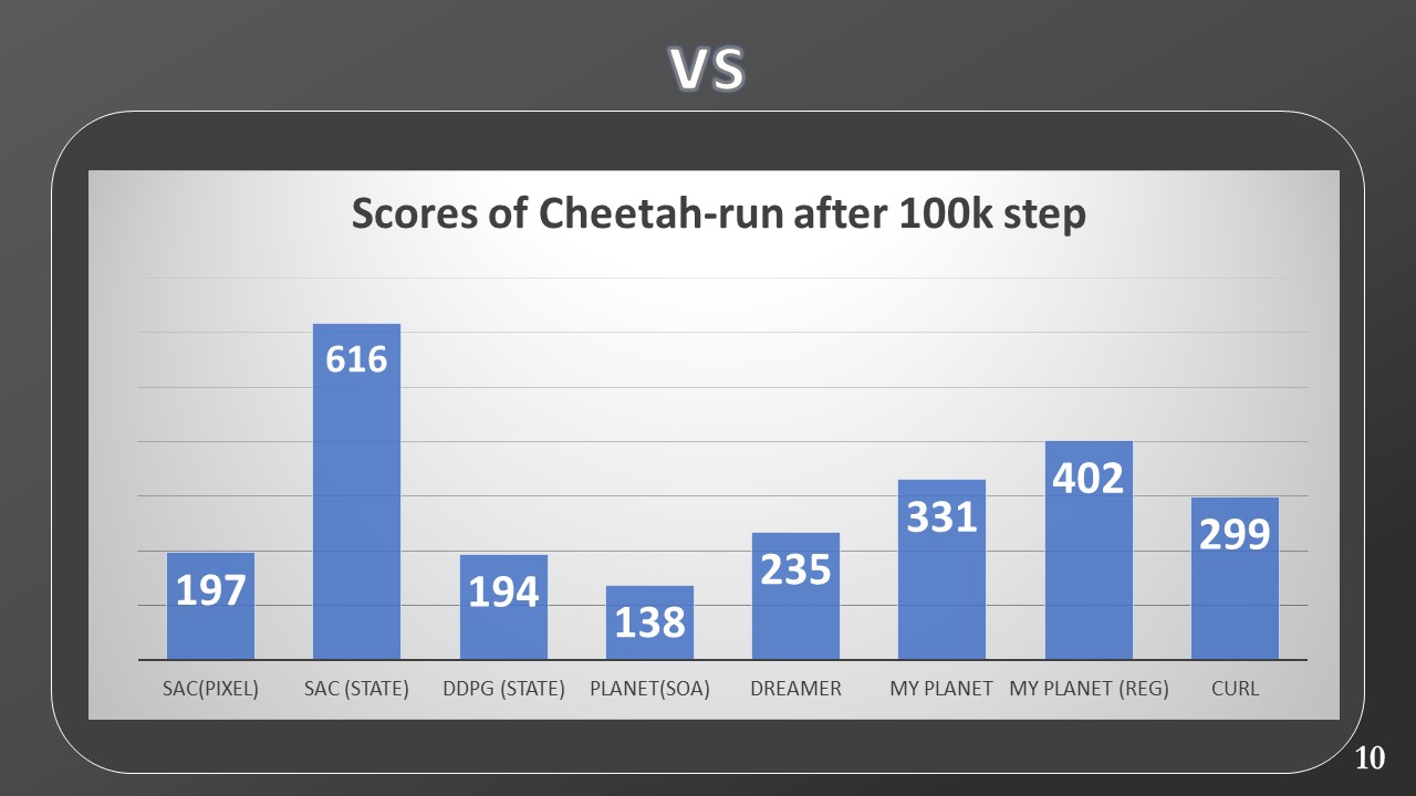
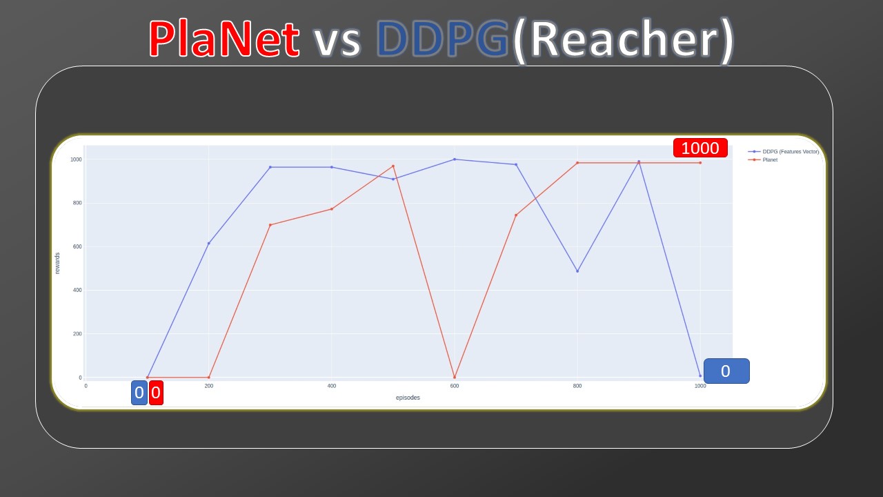
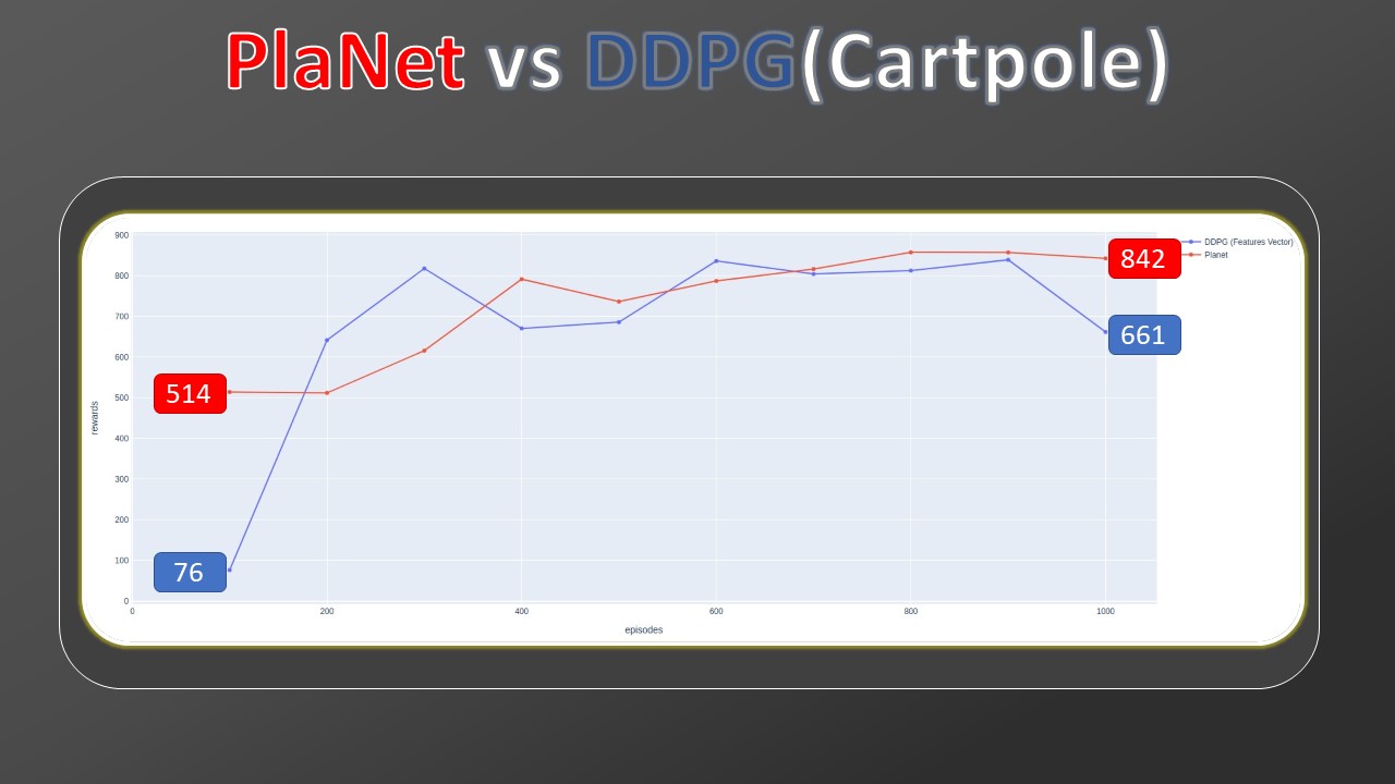
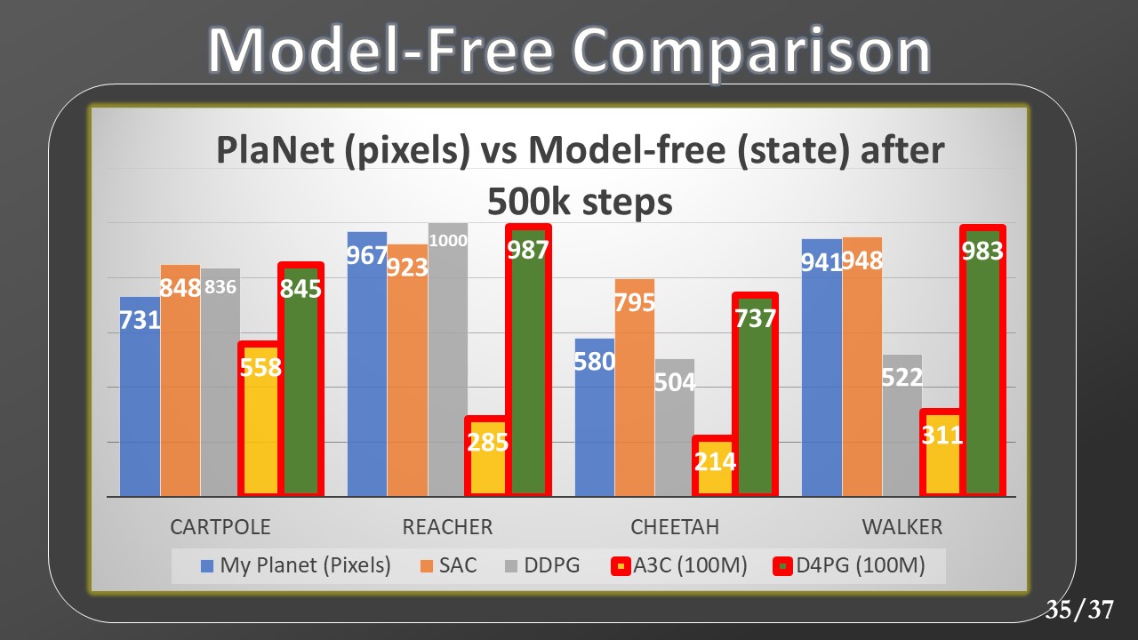 Then, I collected data from other model-free algorithms but this time they are trained through Markov states, while my Planet maintains the training from pixels. For this comparison, we added two more model-free baselines, A3C and DDPG (the latter implemented by myself and part of the thesis work). The bars outlined in red also in this case indicate a training of 100M. By observing the gap between the previous SAC and D4PG and the current ones, we can see how much more complex the training by pixels is, with respect to Markov states. Despite this handicap, Planet's results still remain comparable.
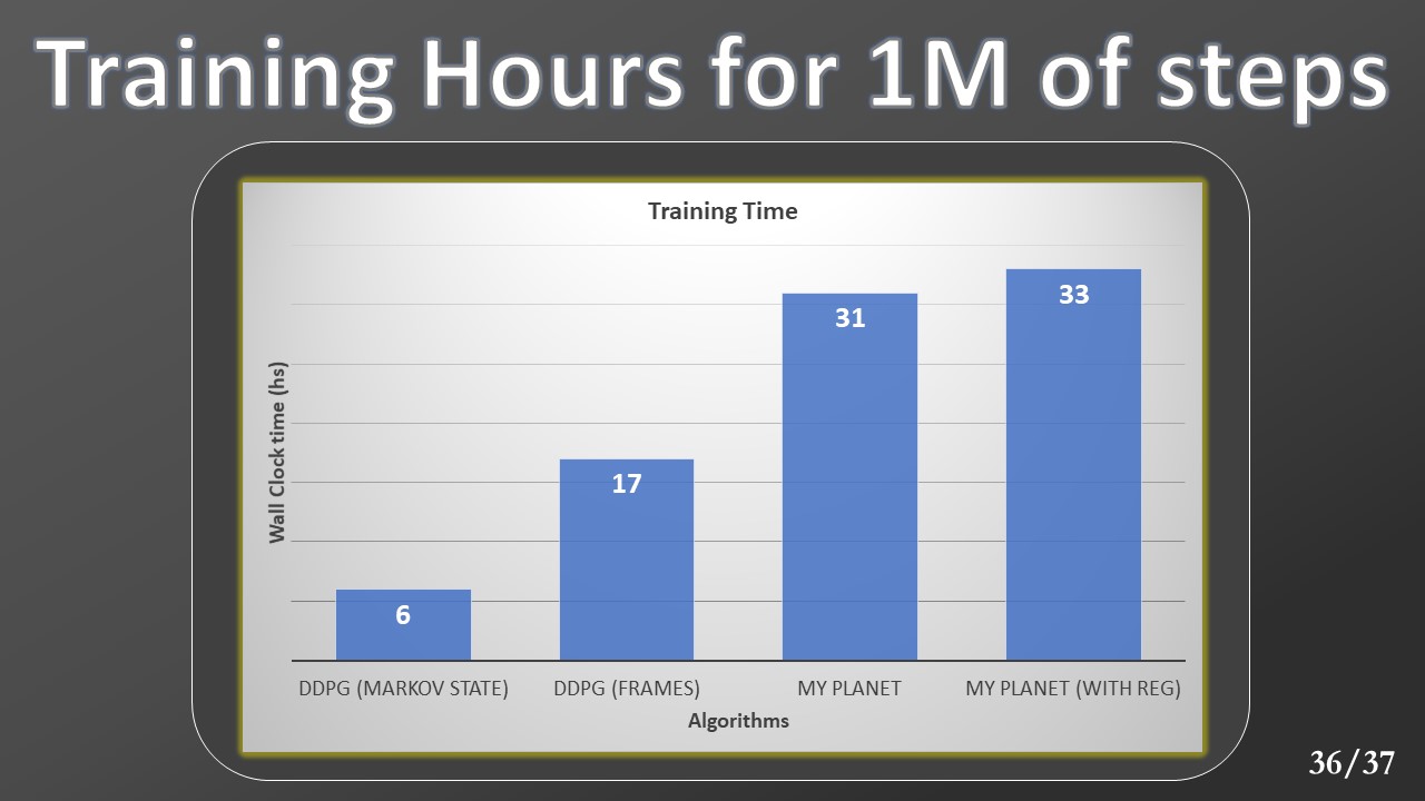 Finally, during the DDPG training, we collect the data relating to training times on a million steps. We can see how the greater complexity of the Planet model leads to slower training, requiring more hours of training.
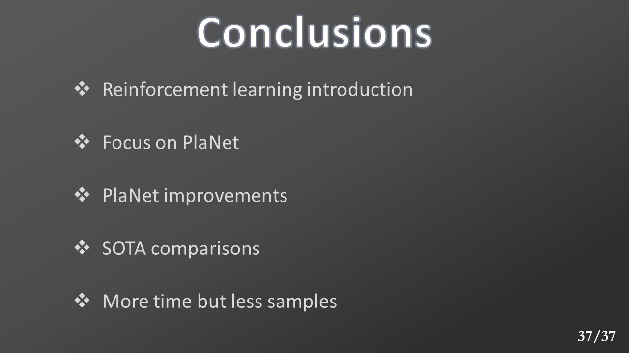 We started by introducing the basic concepts of reinforcement learning.
We have seen how Planet is able to approximate the Markov state and use it to make predictions.
We have seen the results of the improvements introduced.
And finally, we saw a comparison of the results produced with respect to the state of the art
We can conclude that with model-based algorithms, it is possible to obtain performances comparable to those of model-free algorithms with a number of sample orders of magnitude lower at the price of a longer training time.
We started by introducing the basic concepts of reinforcement learning.
We have seen how Planet is able to approximate the Markov state and use it to make predictions.
We have seen the results of the improvements introduced.
And finally, we saw a comparison of the results produced with respect to the state of the art
We can conclude that with model-based algorithms, it is possible to obtain performances comparable to those of model-free algorithms with a number of sample orders of magnitude lower at the price of a longer training time.
 Before concluding, I thank my two supervisors for their valuable advice and Addfor for hosting me.
 Finally, we leave the references from which we collected the data and the main algorithms used.

Italian Video presentation:
[Medium] Deep RL: a Model-Based approach:
Part 1: Deep Reinforcement Learning doesn’t really work… Yet
Part 2: Model-based Deep Reinforcement Learning explained
Part 3: The Deep Planning Network (PlaNet)
Part 4: Our quest to make Reinforcement Learning 200 times more efficient